Cross-hole test

The cross-hole test measures the time P and S waves take to travel from a source borehole to one or more receiver boreholes, with source and receivers at the same depth. Repeated at successive depths, it gives a velocity profile in which each value belongs to a horizontal layer crossed by the waves. The technical reference is ASTM D4428/D4428M.

In Downhole NX the cross-hole is a second test type: traces, time picking, elastic parameters, V_s,eq, stratigraphy, report, DXF, assistant and credits are the same as for the down-hole test.

When to use it

• When you need the horizontal velocity of the layers at given depths, without the oblique path of the down-hole test and without the shallow layers entering the deep travel times.
• When layers are thin compared with the depth but not thin compared with the borehole spacing: with boreholes 3 m apart, a 50 cm layer is skipped by the refracted wave (see Flagged depths).
• With two receivers or more: the interval velocity between two receivers removes the trigger delay, and it is the one the standard recommends.

New cross-hole test

File → New cross-hole test creates a project with a source borehole S and two receivers R1 and R2 in line, 3 m apart, vertical. You can also change the Test type in the General data: the tabs adapt and the data of the other type stay in the project, ready if you switch back.

In a cross-hole test the Boreholes tab replaces the down-hole geometry; Traces, Measurements, Processing, Stratigraphy and Report are still there, adapted to the test.

Boreholes and the deviation survey

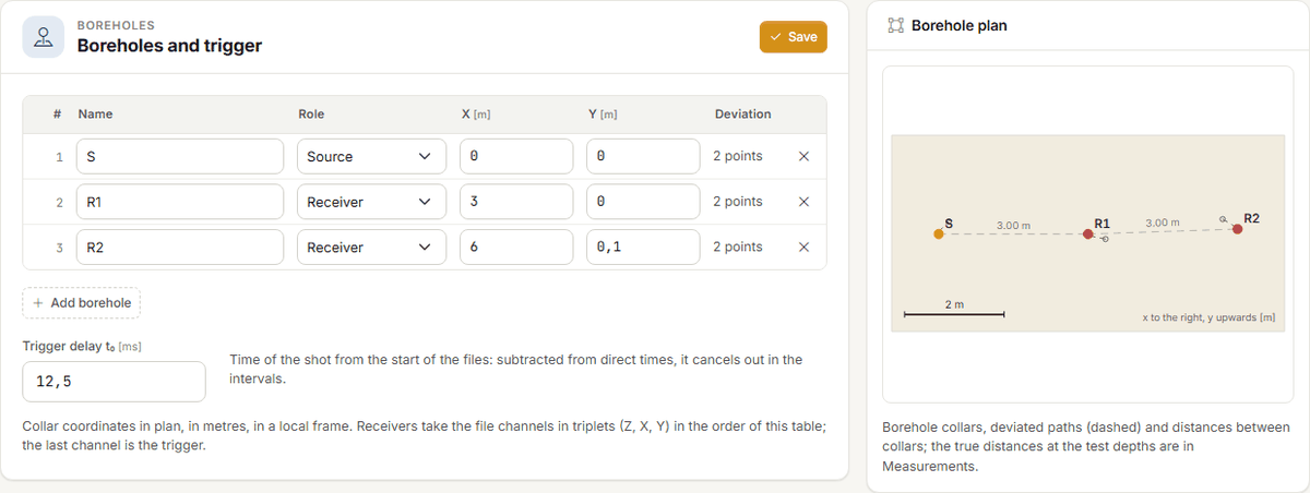
In the Boreholes tab enter, for each borehole, its name, its role (one source, one or more receivers) and the plan coordinates of the collar, X and Y in metres in a local reference. Below the table is the Trigger delay t₀: the instant of the shot relative to the start of the files. It is subtracted from the times of the direct velocities and cancels out in the interval velocities.

The order of the receivers matters

In files with triaxial channels the receivers take channels 1–3, 4–6, … (Z, X, Y) in the order of the table; the trigger is the last channel. A receiver you add goes last.

The Borehole plan, on the right, is redrawn while you type: collars, deviated paths (dashed) and distances between the collars.

Why the survey matters

Boreholes are never perfectly vertical, and velocity is distance divided by time: if the distance is wrong, the velocity is wrong in the same proportion. A receiver 3 m from the source that has drifted 60 cm away at 20 m is actually 3.60 m away: with the same 18 ms, ignoring the deviation gives 167 m/s instead of 200, 17 % less (case 10 in Validation). A borehole without a survey is taken as vertical, and the report says so.

Importing or pasting the survey

Below the plan, in the Borehole deviations card, each borehole has its own table: at vertical depth z the borehole is offset by Δx, Δy from the collar. Between two points the offset is interpolated, below the last it stays the last one. You can type the points, or press Import or paste the survey:

1. choose the Format:
   • z; Δx; Δy in metres — offsets from the collar in metres;
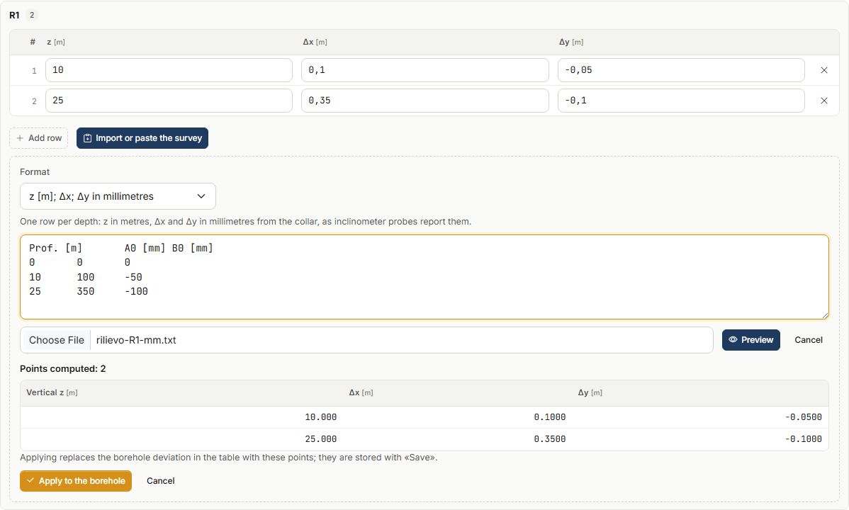
   • z [m]; Δx; Δy in millimetres — as inclinometer probes report them;
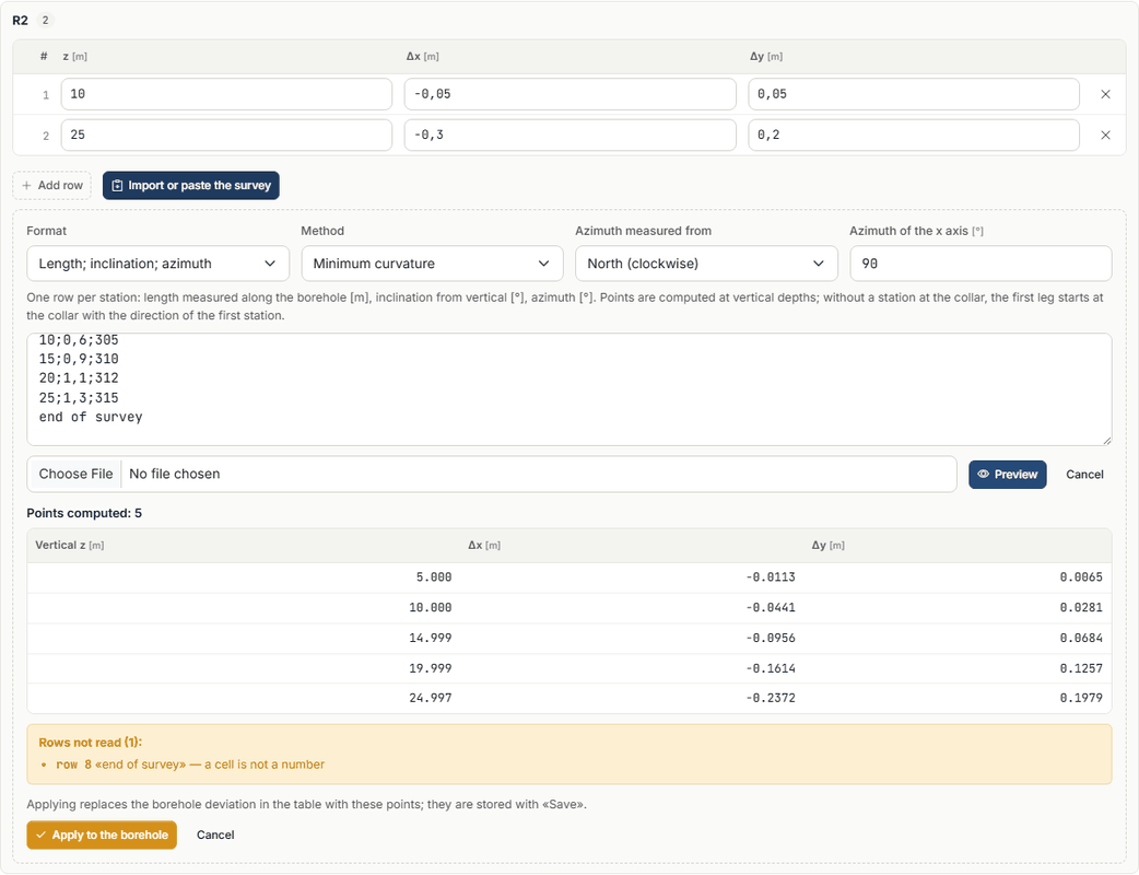
   • Length; inclination; azimuth — one row per station: length measured along the borehole [m], inclination from vertical [°], azimuth [°];
2. paste the rows in the box, or choose a .csv, .txt or .dat file (it is read in the browser, not uploaded);
3. press Preview: you see the computed points and the rows that cannot be read, with the reason;
4. Apply to the borehole puts the points in the borehole table; they are stored with Save.

Accepted separators: semicolon, tab, comma or spaces; the decimal comma is fine. A first row with the column names is skipped, and so is the collar row (0; 0; 0).

With azimuth and inclination also choose:

• the Method: Minimum curvature (between two stations the borehole is a circular arc; the usual method) or Balanced tangential (half the leg with the direction of the upper station, half with that of the lower one);
• what the azimuth is measured from: North, clockwise, or the Site x axis towards y;
• with north, the Azimuth of the x axis of the site: 90° if the x axis points east (then y points north).

Points are computed at vertical depths. If the survey has no station at the collar, the first leg starts at the collar with the direction of the first station.

Millimetres read as metres

A row whose offset is larger than its depth is not read: it is almost always millimetres with the metre format. The same for an inclination over 60° (swapped columns or another unit). The preview lists them before they enter the project.

Traces and times

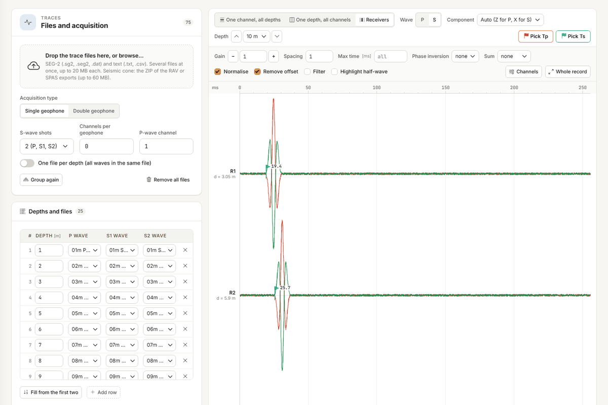
The Traces tab works as in the down-hole test (see Traces and time picking): load the SEG-2 files, one per depth and shot («10m P», «10m S1», «10m S2»), and the app groups them by depth. The cross-hole test adds the Receivers view: one depth, one trace per receiver in order of distance from the source, with the true distance written next to it (d = 3.05 m).

It is the only view where a trace belongs to a receiver, so that is where times are picked: Pick Tp and Pick Ts, then a click on the trace. Component chooses the channel to look at: automatically Z for P and X for S.

The visual check

In order of distance the first arrivals of a depth must lie on a straight line. A receiver off the line has a wrong time, or a refracted wave arrives there first.

Propose the times proposes the first arrivals for every depth and every receiver. Receivers beyond the nearest one are proposed by cross-correlation between receivers: the time of the nearest one plus the delay that makes the two waveforms match. That is how the time difference, and so the interval velocity, is measured well even when the onset of the wave is not sharp. Doubtful times are marked «?» and must be checked; a time you picked by hand is not touched unless you ask to replace it.

P waves between close boreholes

Between boreholes 3 m apart P waves travel in 1–2 ms. With traces sampled at 8 kHz the onset reading can be off by a few tenths of a millisecond, and the direct velocity to the first receiver is affected. The standard asks for 20–50 kHz. Cross-hole times are stored to 0.01 ms.

Measurements

The Measurements tab has one row per depth, with T_p and T_s for each receiver in milliseconds from the start of the files (the calculation removes the trigger delay) and, with the unit weight entered by hand, γ. An empty cell is a time not picked. Below, read only, the true distances at the depth and the direct velocities.

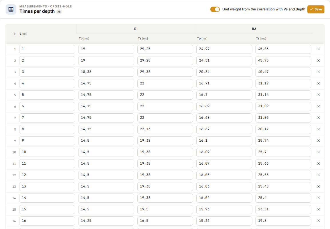
Times arrive in three ways:

• from the Traces tab with Bring in the picked times (the strip at the top offers it when there are times to bring, and warns if it would replace times already written);
• typed;
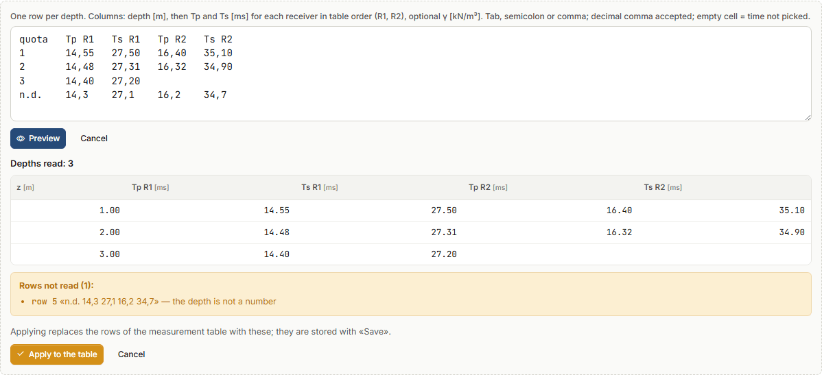
• with Paste from spreadsheet: columns depth, T_p R1, T_s R1, T_p R2, T_s R2… in the order of the receivers in the table, optional γ at the end. Tab (Excel, LibreOffice), semicolon or comma; decimal comma accepted; empty cell or «-» = not picked. Preview shows the depths read and the rows discarded with the reason; Apply to the table replaces the rows of the table. Pasting a block of cells straight into the table opens the same preview.

Processing

For each depth the app computes:

• the true distance between source and receiver, from the deviated points of the boreholes at that depth;
• the direct velocity source → receiver, V = d / (t − t₀);
• the interval velocity between two consecutive receivers in order of distance, V = (d₂ − d₁) / (t₂ − t₁): the trigger delay cancels out. It holds for roughly aligned boreholes, as the standard prescribes;
• the adopted velocity: the mean of the intervals if there are any, otherwise the direct velocity of the nearest receiver;
• the dynamic elastic parameters (γ, ν, G, E_d, E, E_v) with the same formulas as the down-hole test;
• the V_s,eq between the two chosen depths: each depth represents the layer between the midpoints to the neighbouring depths, the first starts at ground level, the last is extended to H if the test is shorter, and this is stated.

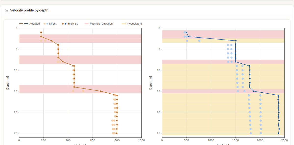
The Velocity profile by depth shows the adopted V_s and V_p (line), direct and interval values (dots), and the bands of the flagged depths.

Flagged depths

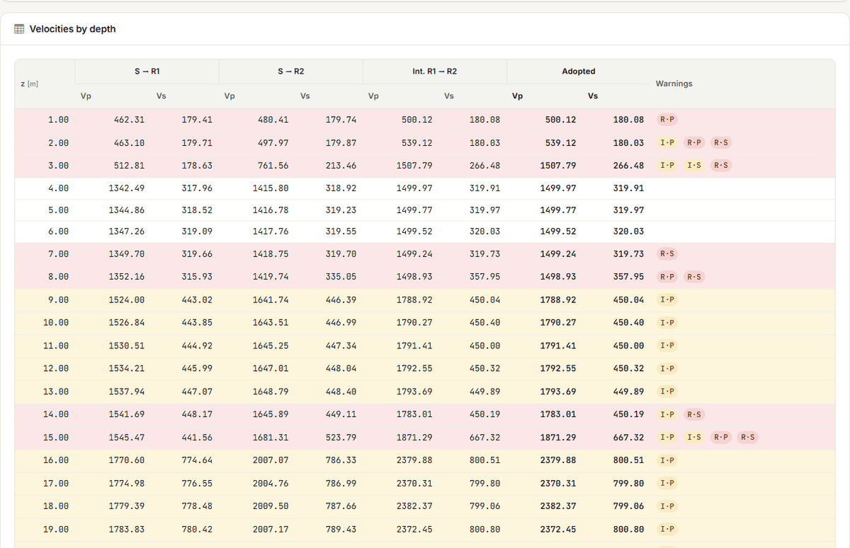
The Velocities by depth table lists direct, interval and adopted values, and the Warnings column has the codes:

Code	Meaning	What to do
R·P, R·S	possible refracted wave: with the profile obtained, the wave refracted along a faster nearby layer would reach one of the receivers before the direct wave	the measured velocity may be that of the fast layer, not of the depth: look at the traces in the Receivers view (versus distance the refracted wave has the slope of the fast layer), and if so do not use that velocity without confirmation
I·P, I·S	inconsistent: the velocities of the pairs at the depth (S → R1, S → R2, R1 → R2) differ by more than 15 %	check the times of the depth and the trigger delay again; often it is the direct velocity to the first receiver, which depends on the onset reading and on t0

Near a velocity contrast the refraction check flags one depth too many, never one too few: this is intended. Flagged depths stay in the calculation and in the V_s,eq (which uses the adopted velocities of all depths): look at them before signing.

Report and DXF

The Report tab works as in the down-hole test (see Report, DXF and credits). For the cross-hole test the report contains the theory of the test, the input data (boreholes, deviations, plan, measurements), the processing by depth (distances, direct and interval velocities, adopted values, flagged depths with their warnings, profile, parameters, V_s,eq), the stratigraphy and the Calculation code block. The DXF drawings are plan, profile and column.

Generating the Word file and exporting the DXF cost credits as in the down-hole test; processing, charts and preview are free.

Assistant

The assistant reads the cross-hole project and results (flagged depths with the reason) and writes into the project, as in the down-hole test, only what you ask:

• the boreholes (name, role, collar coordinates) and the trigger delay: boreholes it does not mention stay as they are;
• the deviation of a borehole as a z, Δx, Δy table in metres; for a survey by azimuth and inclination it asks you to import it from the Boreholes tab, which computes it;
• the times by depth and receiver: it adds depths and times, deletes nothing, and a value already written and different stays until you tell it to replace it;
• the proposal of the times on the traces and their transfer to the measurements, with the same rules as the buttons.

It deletes nothing: you remove boreholes, depths and times yourself. Each message costs credits.

Limits

• Thin layers compared with the borehole spacing: the refracted wave skips them, and the depth is flagged.
• Non-aligned boreholes in the interval method: the difference of the distances is the path between the receivers only if they lie on the same ray from the source.
• Boreholes without a survey: taken as vertical (case 10 shows how much it matters). Below the last survey point the offset stays that of the last point.
• The minimum curvature method is exact on a circular arc; on a nearly vertical borehole with a turning azimuth it is off by fractions of a millimetre (case 14).
• Anisotropy (horizontal versus vertical V_s) is not handled.
• Proposed times are proposals: S waves hold even between close boreholes, P waves depend on the sampling.
• As in the down-hole test: dynamic moduli, at small strains; the subsoil category is up to the designer.

---

Found an error on this page? Let us know or open a Pull Request.