Rainfall depth-duration-frequency curve

The curve links the rainfall depth to the event duration for a given return period. It is the input of every sizing method.

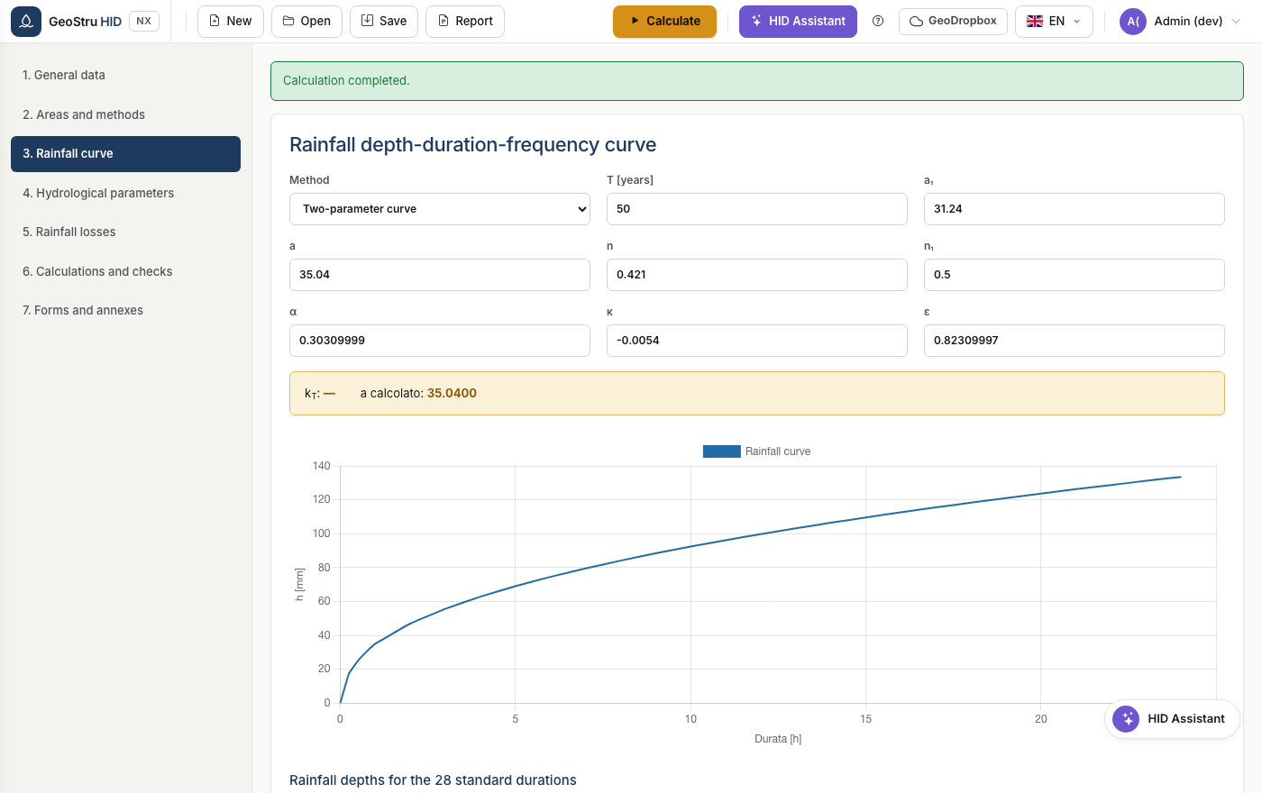
Two-parameter curve

The classic form:

\[h(t) = a \cdot t^{n}\]

with h in mm and t in hours. Enter a (hourly rainfall coefficient) and n (scale coefficient). The parameter n₁ governs durations shorter than one hour, where the curve has a different slope; the usual value is 0.5.

Example

With a = 46.49 and n = 0.364 the 3-hour rainfall is 46.49 × 3^0.364 = 69.35 mm; the 24-hour rainfall is 147.83 mm.

GEV curve

The generalised extreme value distribution derives the coefficient a from the hourly coefficient a₁ and from the growth factor linked to the return period:

\[a = a_1 \cdot K_T\]

Enter the parameters α (alpha), k (kappa) and ε (epsilon) and the return period. HID calculates K_T and shows it next to the curve.

Lombardia

The regional regulation requires the GEV curve. The parameters are obtained from the reference regional service. With the two-parameter curve HID blocks the calculation.

Table and chart

After the calculation the table shows the depths at the 28 standard durations: 0, 0.25, 0.50, 0.75, 1 hour, then every hour up to 24. The chart below shows the same series.

Rounding

Values are calculated in double precision and rounded only for display. Small differences in the last digit compared with other software depend on the rounding direction, not on the calculation.

---

Found an error on this page? Let us know.